Those that are familiar with PowerPivot and DAX, will be aware that DAX provides the ability to reference columns.
However, it does not provide support for Cell based references (such as A1, E23).
This is normally no big issue, until I hit a small design issue this week… I had the requirement to refer to a previous row of data within the PowerPivot model.
And yes, it is possible, using the EARLIER DAX function.
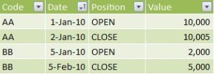
Let me talk through the data quickly… I received some stock futures trading data, where each trade had two rows. One row would be the opening position at a point in time, and when the future actually closed, a second row would come through with the closing position. The profit made would be the difference between the opening position and the closing position.
Something like the following table…
The basic process to solve this problem was to do the following:
1. for every row, determine the Previous Date that applies to this particular Client Code.
2. Once the Date is established, determine the Value at that point in time.
3. Profit is then simply Current Value – Previous Value for CLOSE rows.
1. Using the following DAX statement, I could calculate the [DatePrevious] column
=CALCULATE(MAX(Table1[Date]), (FILTER(Table1, EARLIER(Table1[Code])=Table1[Code] && EARLIER(Table1[Date])>Table1[Date])))
Note: I’m still coming to grips with the EARLIER function, seems to work semantically the same as an INNER join… will hopefully post a better explanation when I understand some more…
2. Using similar thinking, I could then join back to [Table1] and return the Value at the point in time established in the previous step.
(I would love any feedback if it’s possible to merge this with the previous step, may be more efficient)
=CALCULATE(SUM(Table1[Value]), (FILTER(Table1, EARLIER(Table1[Code])=Table1[Code] && EARLIER(Table1[DatePrevious])=Table1[Date])))
3. Finally, Profit is then just the difference between the current value and the previous value for the CLOSE rows.
=if(Table1[Position]="CLOSE", Table1[Value]-Table1[ValuePrevious], BLANK())
Results in the table below.


#1 by David Hager on March 20, 2011 - 10:05 pm
You can use:
=CALCULATE(MAX(Table1[Value]),(FILTER(Table1,EARLIER(Table1[Code])=Table1[Code] && EARLIER(Table1[Date])>Table1[Date])))
to replace the two calculated columns.
BTW, great stuff!
#2 by jsimonbi on March 28, 2011 - 4:40 am
Good stuff Gavin.
#3 by David Hager on March 31, 2011 - 4:24 pm
Gavin,
See:
http://powerpivotpro.com/2011/03/31/guest-post-nth-occurrence-dax-formula/
#4 by Martin on April 17, 2011 - 4:11 pm
Generally, this can be done by the PivotTable quite easily.
No DAX such stuffs
#5 by Gavin Russell-Rockliff on April 18, 2011 - 8:47 am
Fair call, it is possible to setup measures in the pivot, using standard excel calculations, that may be similar. However, this would normally involve displaying the lowest level data in the pivot, and sorting by key and date? In my mind, it may be quite tough to get an aggregated sum?
Would love to see how you would achieve this without Dax.
Also, in principle, i’m always a fan of putting logic as deep as possible to allow for reuse across pivots and any other report or model that uses this power pivot logic. Defining calcs in the pivot, in the excel sense, would not allow reuse of these measures.
#6 by Pedro on July 28, 2011 - 12:00 pm
I was trying to understand the earlier function , by reading this http://social.technet.microsoft.com/wiki/contents/articles/powerpivot-dax-filter-functions.aspx#earlier, but I still don’t get it.
Specifically in this part:
A new calculated column, SubCategorySalesRanking, is created by using the following formula.
= COUNTROWS(FILTER(ProductSubcategory, EARLIER(ProductSubcategory[TotalSubcategorySales])<ProductSubcategory[TotalSubcategorySales]))+1
The following steps describe the method of calculation in more detail.
The EARLIER function gets the value of TotalSubcategorySales for the current row in the table. In this case, because the process is starting, it is the first row in the table
EARLIER([TotalSubcategorySales]) evaluates to $156,167.88, the current row in the outer loop.
The FILTER function now returns a table where all rows have a value of TotalSubcategorySales larger than $156,167.88 (which is the current value for EARLIER).
The COUNTROWS function counts the rows of the filtered table and assigns that value to the new calculated column in the current row plus 1. Adding 1 is needed to prevent the top ranked value from become a Blank.
The calculated column formula moves to the next row and repeats steps 1 to 4. These steps are repeated until the end of the table is reached.
could you please describe in the example above, wat is the inner and the outer loop? And could you please describe what happens in these four steps for the second row.
I thought that the earlier function returned the value from the previous row, but I can see that it's more complicated than that. To check this I created a very simple table , and then I added a calculated column just with the earlier function , to see if the value from the previous row was returned, but I got errors.
Thanks in advance